Table of contents
- What is atmospheric refraction?
- What does the amount of refraction depend on?
- Influence of refraction on distant views
- Effect of refraction on visibility range
- Refraction in visibility simulations
What is atmospheric refraction?
This is the refraction of light in the air resulting from changes in atmospheric density with altitude. These in turn are caused primarily by changes in atmospheric pressure and air temperature.
Light in the Earth’s atmosphere does not normally run in a straight line – this would be the case in a vacuum. According to Snellius’ law, the direction of the light beam changes at the boundary between media with different refractive indices. This is exactly the same phenomenon that can be observed at the boundary between air and water or air and glass, e.g. in lenses. Here, however, there is no sharp boundary between the media – the changes in the properties of air are smooth, so instead of a sudden change in the direction of the light ray, there is a gradual, gentle curvature over a long distance.
Atmospheric refraction always occurs, with two exceptions – vertical observations (light is not refracted when it falls perpendicular to the boundary surface between the media) and when there is a strongly increased vertical thermal gradient, such as over a body of water warmer than the air. In the latter case, the decrease in atmospheric density associated with changes in pressure is offset by an increase in density due to decreasing temperature.
Its measure is the the coefficient of refraction, defined as the ratio of the Earth radius to the radius of the light ray curvature. Its local value is given by the following formula:

where p – atmospheric pressure in hPa, T – air temperature in kelvins, dT / dh – vertical temperature gradient per 1 m altitude difference (in K/m). It can be calculated using this spreadsheet. Its derivation can be found, for example, on Walter Bislin’s website. This is a simplified formula, not taking into account factors that affect refraction to a small extent, such as air humidity.
What does the amount of refraction depend on?
The biggest influence on the value of the coefficient is the vertical temperature gradient, i.e. the rate of change of air temperature with altitude. By default, it results from the adiabatic transformation occurring in the compression and expansion of air that accompany changes in altitude (the higher the altitude, the lower the atmospheric pressure) and is about -0.65 °C/100 m if condensation occurs during ascent, and about -1 °C/100 m in dry air when condensation does not occur. However, the temperature distribution depending on altitude can change, for example during a temperature inversion, when the air becomes warmer with increasing altitude. Then the gradient can reach several degrees per 100 m, its numerical value is positive (under standard conditions it’s negative). In long distance observations several types of inversion are important.
- Subsidence inversion – occurs in high-pressure areas, as a result of descending air movements that warm adiabatically, becoming warmer than the air layer below. In Poland it is encountered in the mountains and sometimes in the foothills, especially in winter. The air falling downwards is very dry, clean and has exceptionally good visibility, but the layer below is characterised by reduced transparency, with a high concentration of pollution and often moisture. Therefore, in the area of influence of a strong baric high, distant views are often difficult at low altitudes, while a few hundred metres above, visibility can reach hundreds of kilometres.
- Radiative inversion – is created by radiating heat from the ground during cloudless and windless weather at the end of the day and at night. The layer of air close to the ground cools faster than the air above. This type of inversion particularly affects observations in regions with little relief, where the line of sight runs low above the ground for a long distance.
- Advective inversion – occurs when warmer air flows over cooler ground. Like a radiation inversion, it affects the near-ground air layer. It can occur over bodies of water.
The value of air temperature itself is also important – refraction is stronger in cooler air.
The effect of atmospheric pressure on the variation of refraction at a given location is relatively small – pressure changes at a constant altitude are not large. It is, however, an important factor when considering refraction at high altitudes – as altitude increases, pressure decreases, so the refraction coefficient is smaller.
Air humidity has a noticeable effect on refraction if it changes strongly with altitude – for example, over water.
When typical values encountered in the Polish climate are inserted into the above-mentioned formula, the results are higher than those considered average of 0.13-0.14. At a vertical temperature gradient of -1 °C/100 m (a typical value for dry air) and a pressure of 1013 hPa, the value of 0.13 occurs at 35 °C. These calculations suggest that in Polish climate the values are slightly higher, in the region of 0.15-0.17.
Example values for different conditions (a minus next to the thermal gradient indicates a decrease in temperature with increasing altitude):
| temperature [°C] | temperature gradient in °C per 100 m | pressure [hPa] | refraction coefficient |
| 20 | -0.65 | 1000 | 0.163 |
| -10 | -0.65 | 1000 | 0.202 |
| 20 | -0.65 | 900 | 0.146 |
| 20 | -1 | 1000 | 0.142 |
| 20 | 1 | 1000 | 0.26 |
| 0 | 2 | 1000 | 0.366 |
| 30 | -2 | 1000 | 0.078 |
Influence of refraction on distant views
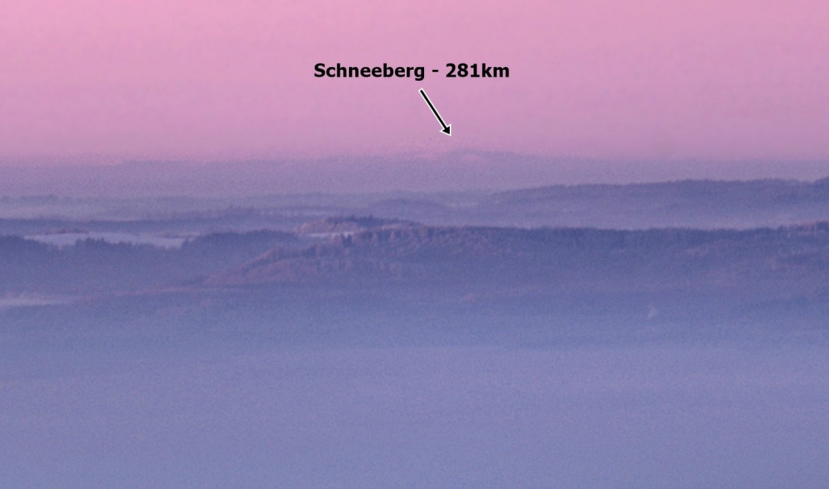
Atmospheric refraction increases the range of visibility and makes it possible to observe objects that would otherwise be hidden behind the horizon. The stronger it is, the more distant objects protrude above the horizon. The importance of atmospheric refraction in long-distance observations concerns mainly the visibility of objects at distances close to the maximum – thanks to increased refraction, observations are possible from places farther away than under standard conditions.
As a result of refraction, the observed object is seen higher than it would be if the light ran in a straight line. The size of this apparent increase in height is given by the following formula, in which h – height of apparent elevation, d – distance, k – refraction coefficient, R – radius of the Earth:

The elevation affects the entire visible landscape, so to determine its value in relation to a closer point, the uplift of a farther point must be subtracted from the uplift of a closer one, multiplied by the quotient of the distances to the farther point and the closer one:
The above formulae contain approximations for small angles – but are sufficiently accurate for distances at which observations from the Earth are possible.
Programs that calculate visibility ranges and simulate panoramas take into account a refraction coefficient of 0.13 in their calculations. As can be seen in the table above, it reaches about 0.14 at a gradient of -1 °C / 100 m at 20 °C, i.e. under typical conditions in dry air in the warm half of the year. For most of the year the temperatures in Poland are lower, so in autumn or winter it is common for this parameter to rise to around 0.17-0.2 in the lower troposphere. The best time to observe Tatra Mountains from the greatest distances in Poland, i.e. from the Lublin Upland and Roztocze, comes in autumn and winter due to the favourable azimuth of the setting sun, and the resulting illumination of the sky at dusk, increasing contrast. It is therefore not surprising that they can often be seen from many locations not recognised by simulations. Theoretically, the best refractive conditions should be at strong frost and cloudless skies, but in Poland, in lowland and highland areas, there is then usually high air pollution, which significantly reduces visibility.
Observations of the Tatra Mountains from the Lublin Upland show that in the cooler half of the year after sunset, the refractive index often reaches values of 0.2-0.22. This is an averaged value calculated on the basis of photographs. Observations in such regions are characterised by a long-distance course of light at a low height above ground level, where a radiation inversion can occur. The photographs show that in this area the value is sometimes even higher (around 0.3 above the forests of the Sandomierz Basin), while farther and higher up it is significantly lower, resulting in a similar effect as if there was a constant refractive index slightly above 0.2 over the entire distance.

Under subsidence inversion conditions in the mountains, there have observed peaks, for visibility of which the average refractive index must be at least about 0.3 (e.g. Heukuppe in Austrian Alps seen from Śnieżnik in Sudetes).
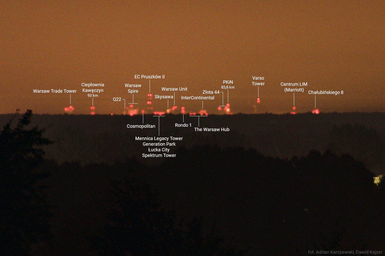
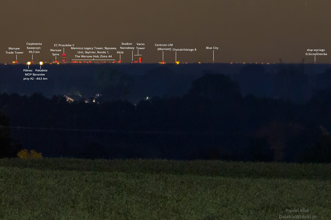
Radiative inversion occurs in a fairly thin layer of air above the ground. For this reason, observations of lower-lying objects can be characterised by a much stronger refractive influence than observations of high mountains, where the light travels a large part of the distance above the inversion. The lights of Warsaw skyscrapers have been photographed from Kalenice near Łowicz, the lowest of which should be visible at a constant refraction coefficient of about 0.8. Sounding measurements of air temperature show that locally this coefficient can reach a value above 1 (analysis of an example measurement from Legionowo in post Warsaw seen from Kalenice).
For observations at distances close to the maximum, when the object is hidden just below the horizon under standard conditions, the refraction coefficient for visibility (assuming it is constant) can be calculated. This can be done with this spreadsheet, using the method described here. It is also possible to calculate the apparent elevation of the horizon under the influence of refraction by using the same spreadsheet.
Refractive inhomogeneities can cause image deformation. In extreme cases, large mirage distortions are visible – this refers to significant refraction changes in thin air layer, which sometimes accompany observations in a strong thermal inversion.
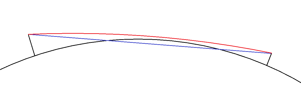
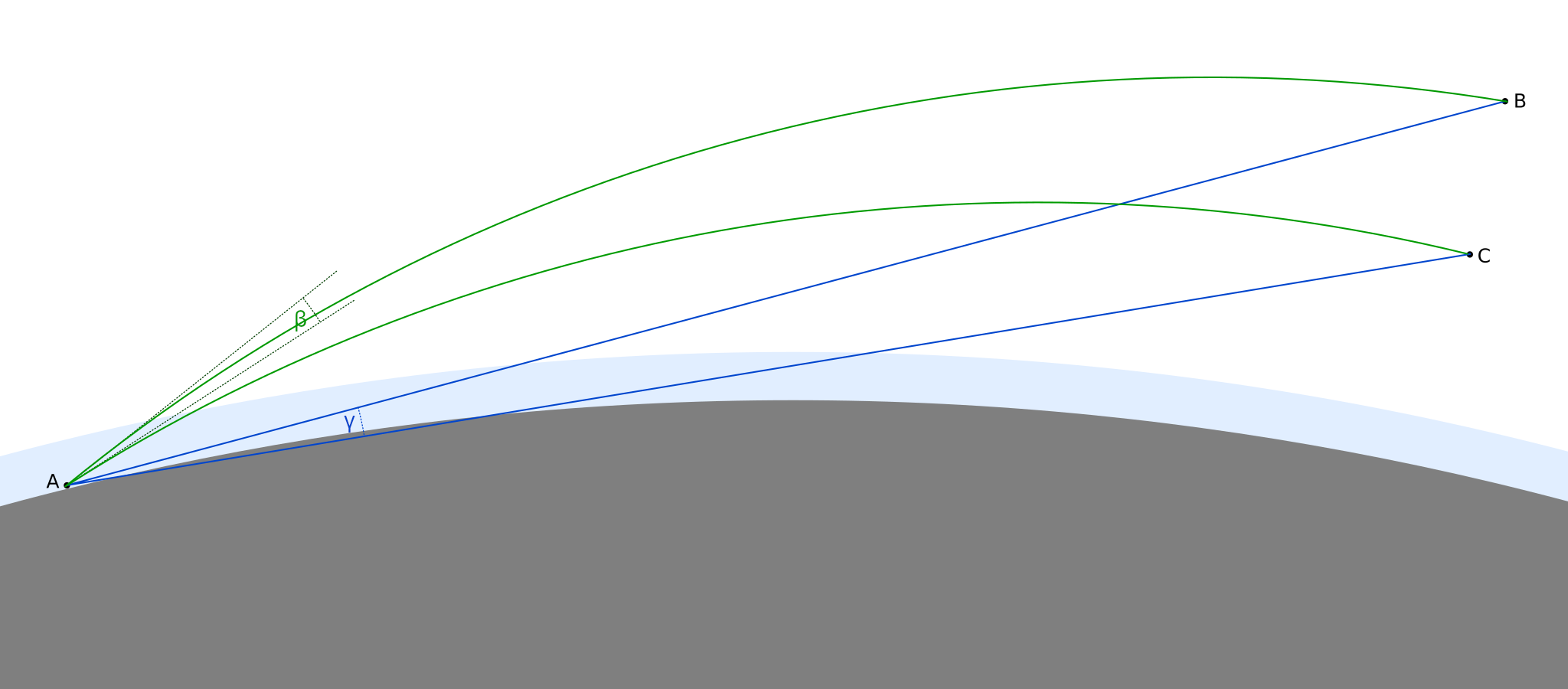
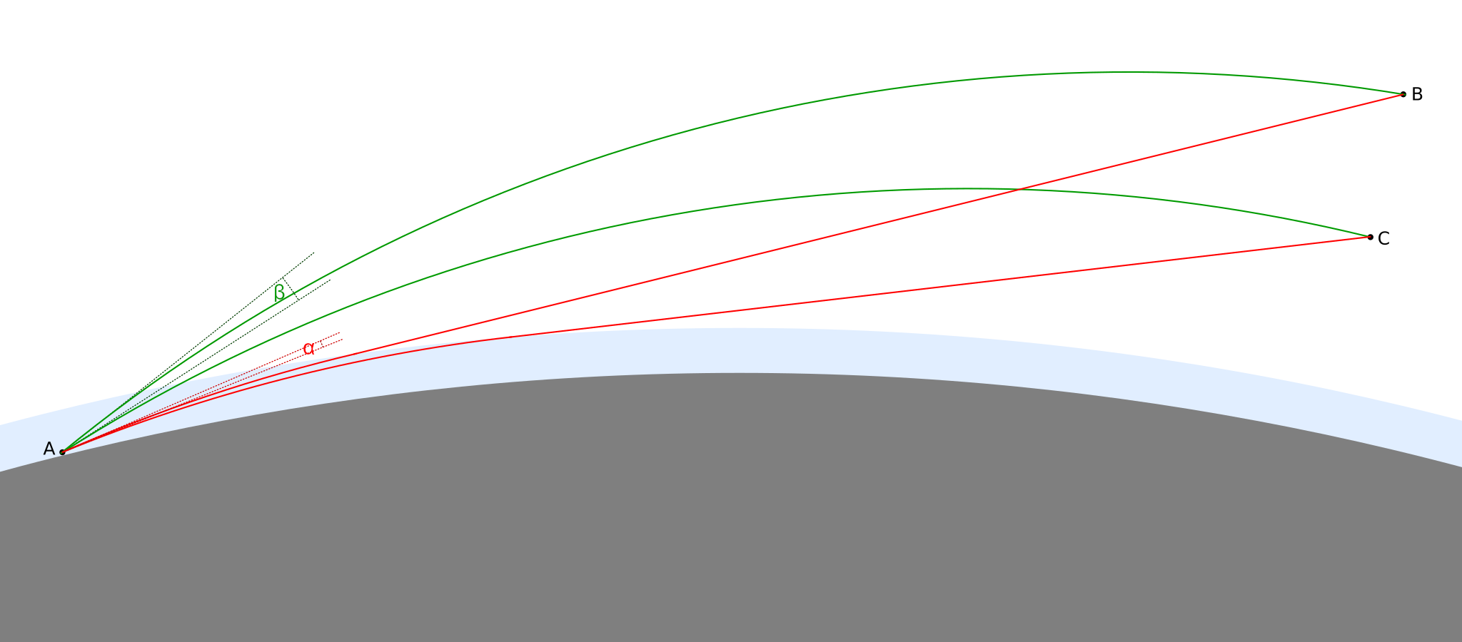
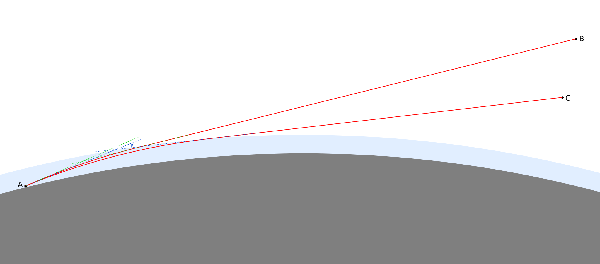
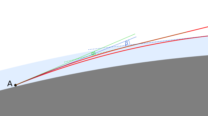
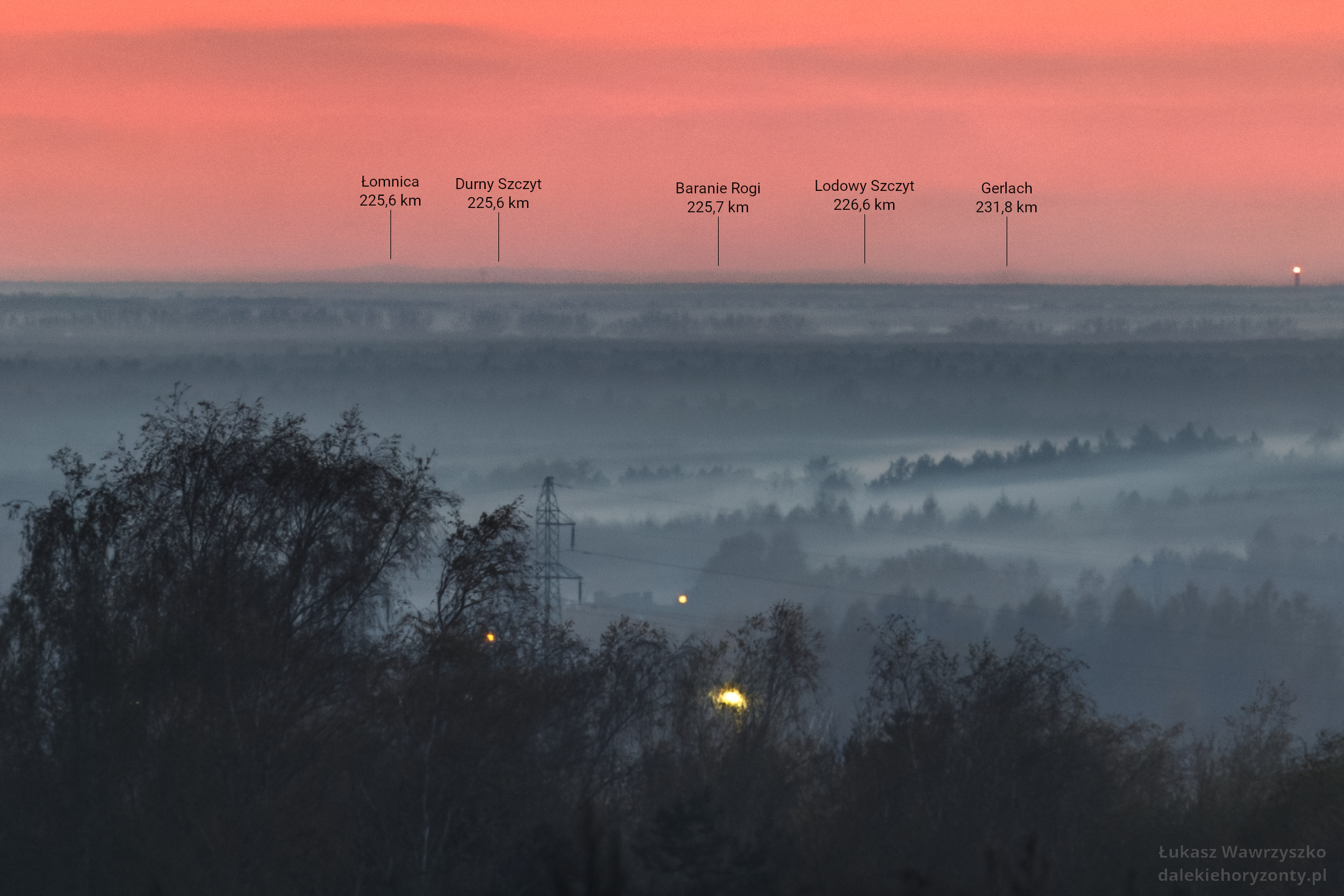
Flattening of the image may also occur – often, to varying degrees, accompanying observations of the Tatra Mountains from the Lublin Upland, where light runs low above the ground for a long distance. When the phenomenon is severe, sharp mountain peaks look like a flat band. This happens with stronger refraction of light in a thin layer of air, where there is an unusual temperature distribution depending on altitude. The angle by which a ray of light is curved depends on the distance it travels through the air. The longer it runs in a layer of air with strong refraction, the more strongly it is refracted. Light travelling from a lower point travels a longer distance within this layer compared to a higher point, and is therefore more strongly curved. As a result there is a distortion of the image of the mountains such that the lower mountain peaks and slopes are raised stronger than higher peaks. The formation of this phenomenon is shown in the figures below.
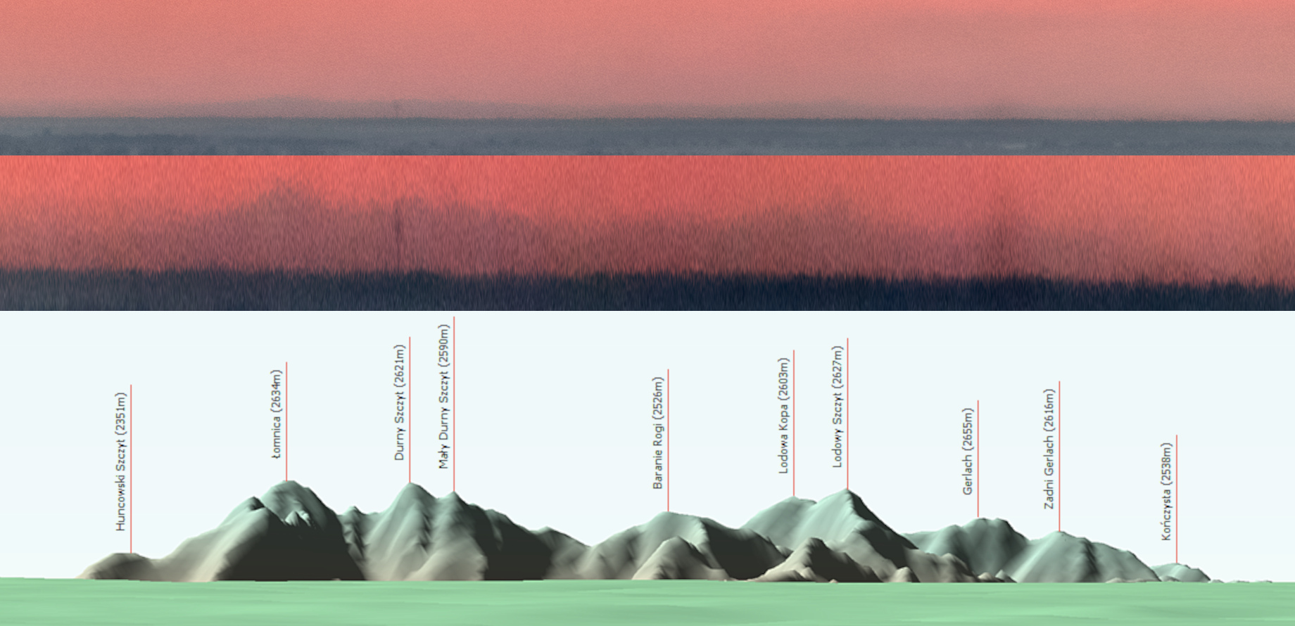
An example is the view of the Tatra Mountains from Łychów Gościeradowski on 3.11.2022. When the photo is stretched vertically, the peaks are more clearly outlined, matching their expected layout.
Effect of refraction on visibility range

where h – observer’s altitude, R – Earth radius.
The table below shows the range of visibility from points 100 and 1,000 metres above the ground for the flat terrain.
| altitude above ground [m] | refraction coefficient | visibility range [km] | percentage range increase |
| 100 | 0 | 35.70 | 0.00% |
| 100 | 0.13 | 38.27 | 7.21% |
| 100 | 0.3 | 42.66 | 19.52% |
| 1000 | 0 | 112.88 | 0.00% |
| 1000 | 0.13 | 121.02 | 7.21% |
| 1000 | 0.3 | 134.92 | 19.52% |
Refraction in visibility simulations
The effect of atmospheric refraction can be represented quite well in some visualisation software for panoramic views if it does not change significantly along the line of sight between the observer and the object seen. The problem arises under conditions that provide a significant increase in refraction, which many distant observers look forward to. This refers to a temperature inversion, which occurs in a layer of air of small thickness. If light travels a relatively large height difference between the object and the observer, part of the distance will travel out of the inversion layer. There is then a significant variation in refraction and vertical distortion of the image occurs, which looks different to that with uniform refraction. The average refractive index calculated from a photograph taken under these conditions then takes on different values for objects of different heights. This cannot be represented by a programme that only allows a single, constant refractive index value to be set.
In programmes that create simulations of view panoramas, it is possible to take atmospheric refraction into account in the following ways:
- accurate calculation of light rays based on the given vertical profile of air temperature and humidity
- increasing the Earth radius
- making simulations from a greater height above ground level
- increasing the observed point height
This method represents the effect of refraction on the entire panorama very well, regardless of the terrain or the distance over which the view extends. It uses the following assumption – mathematically, the effect of atmospheric refraction is as if light ran in a straight line and the Earth had a radius of curvature equal to r = R / (1 – k), where R is the radius of the Earth, k is the refraction coefficient (as mentioned above). It is probably applied in U. Deuschle’s panorma generator. By default, it uses a value of k=0.13, but this can be changed by entering as the simulation range the phrase X_RCY, where X – simulation range in km, Y – refraction coefficient – (e.g. 300_RC0,3 for range of 300 km and refraction coefficient of 0,3).
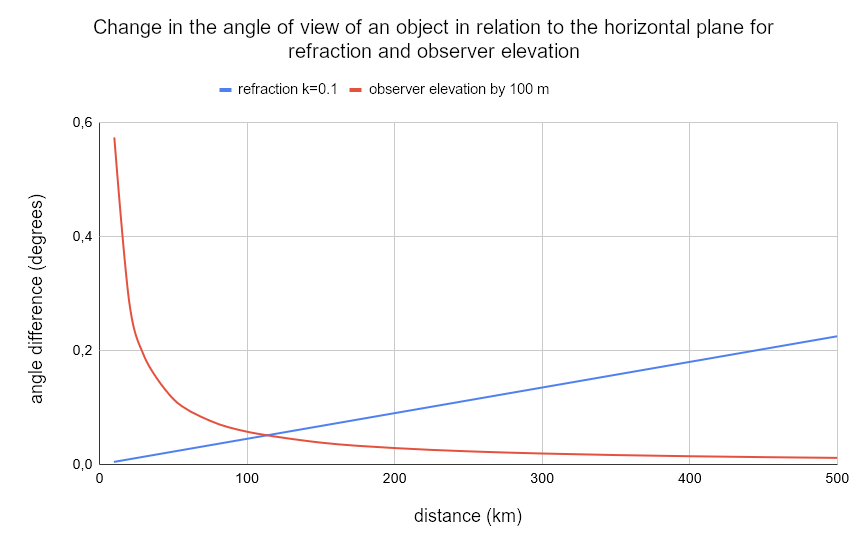
This method works in any software that has the ability to simulate from any height above the ground, but it has a significant drawback. The view from a point raised above the earth’s surface is different from that produced by refraction – the angles relative to the horizontal plane at which the individual elements of the panorama are seen change differently. Refraction makes objects visible higher and this elevation increases with distance. In contrast, when the height of the observer is increased, the angle between the object and the horizontal plane increases less and less with distance – so it is the opposite of the effect of refraction. It is therefore impossible to illustrate the effect of refraction on the entire panorama using this method.
The application of this method is limited to illustrating the apparent increase in height of a visible object in relation to another, closer object – usually it is best to choose the farthest point visible in front of this object. In such a defined arrangement of points it works very well, but it’s important to omit parts of the panorama located at distances significantly different from the distances to these points.
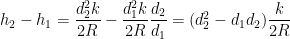
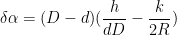
The height by which the simulation location should be raised is determined by an approximate formula:
where k – refraction coefficient (or its difference), d1 – distance to the closer point, in relation to which the apparent lift is determined, d2 – distance to the farther observed object, R – Earth radius.
It can be transformed by introducing the distance ratio n = d2 / d1:
It shows that height is inversely proportional to the ratio of the distance to those two points.


The quantity of error in this method can be determined for each point visible in the simulation by the angle by which the point is displaced in the simulation compared to a simulation that faithfully reflects the effect of refraction. In other words, it is the difference in the angle at which a point is visible on both simulations relative to the horizontal plane for the location where the simulation was performed. The displacement resulting from the difference in these methods occurs always in the vertical direction, the azimuth does not change. The measure of this angle expressed in radians is given by the formula:
where Δα – angle of displacement (elevation) of a point in relation to the correct refraction representation, D – distance to the point in relation to which the displacement is determined, d – distance to the point for which the calculation is performed, h – height of the point from which the simulation is performed, k – refraction coefficient, R – radius of the Earth.
Converting the angle into degrees and then multiplying by the resolution of the simulation in pixels per degree, the value of this offset is obtained in pixels.
The formula is suitable for small angles – for very small distances, comparable to the elevation of the simulation site, the angle is large and a more complicated version of the formula without trigonometric function approximations should be used.
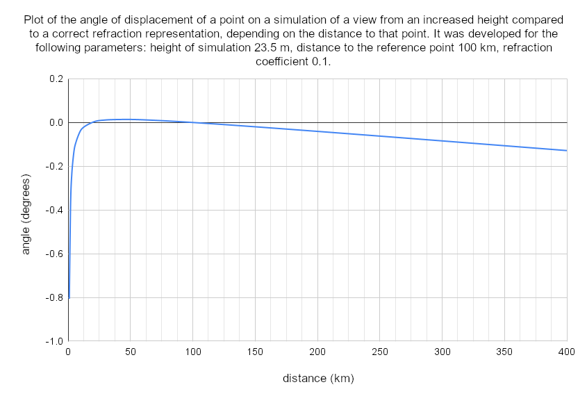
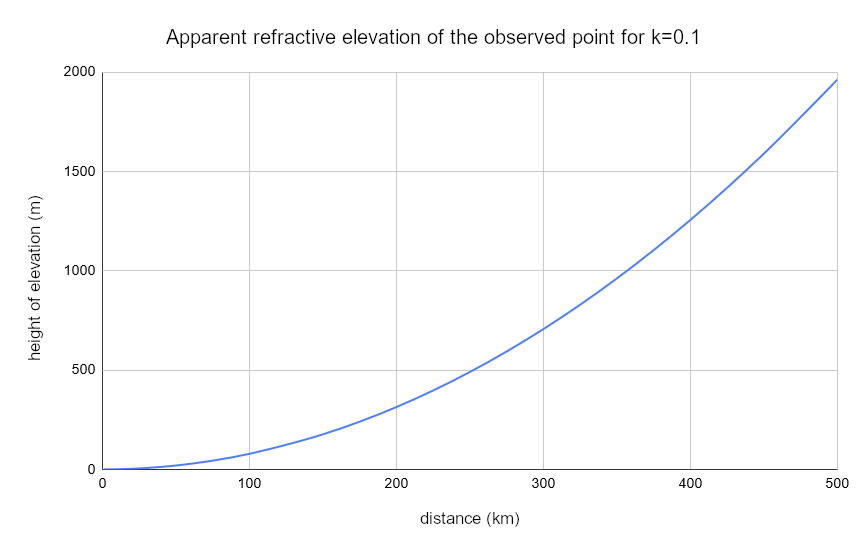
The graph shows the dependence of the method error on distance, specifically the angle of displacement of a point seen from a height of 23.5 m compared to a view with a refraction coefficient of 0.1, this displacement is determined relative to a point 100 km away. This height has been calculated to correspond to the refractive lift of a point 100 km away compared to a point at a distance of 30 km – therefore, the angle is 0 in these points. Returning to the designations in the above-mentioned formulae – in this case d₁ = 30 km, d₂ = 100 km. It is clear from the graph (and formula) that in a simulation for the height H(obs) calculated using the formula above, areas closer than d₁ will be lowered (and this lowering increases rapidly for small distances), between d₁ and d₂ will be elevated, while areas farther away from d₂ are again lowered compared to the actual effect of refraction.
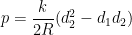
This is useful, for example, in Heywhatsthat to determine areas of object visibility with increased refraction. The situation here is similar to the one discussed above, but the simulation is created in the opposite direction. Alternatively, the elevation of the observed object can be calculated using the formula:
This method, too, should only be considered for a specific observation point – intermediate point – observed point system, the elevation also depends on the ratio of the distance to both these points:

The derivation of the formulae can be found at Calculations.
Let’s see what the effects of the different methods look like in practice using the example of the view of the Tatra Mountains from Potok Wielki in the Lublin Voivodeship, generated by the U. Deuschle’s simulator. For a refractive index of 0.22, the most distant point visible in front of Lomnica lies at a distance of 52 km, while it is 226.5 km to Łomnica. Substituting these data into the formula for the elevation of the observer gives an altitude of 83 m. As the refraction coefficient, you must insert its difference from the default value of 0.13 used in these simulations, i.e. 0.09.
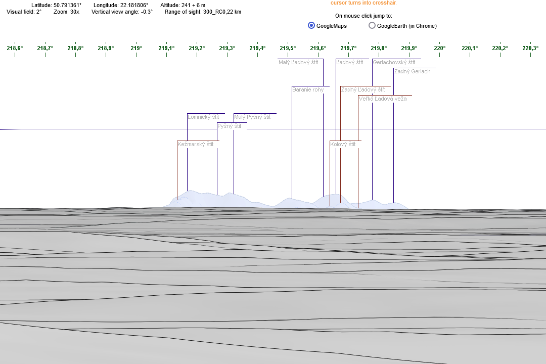
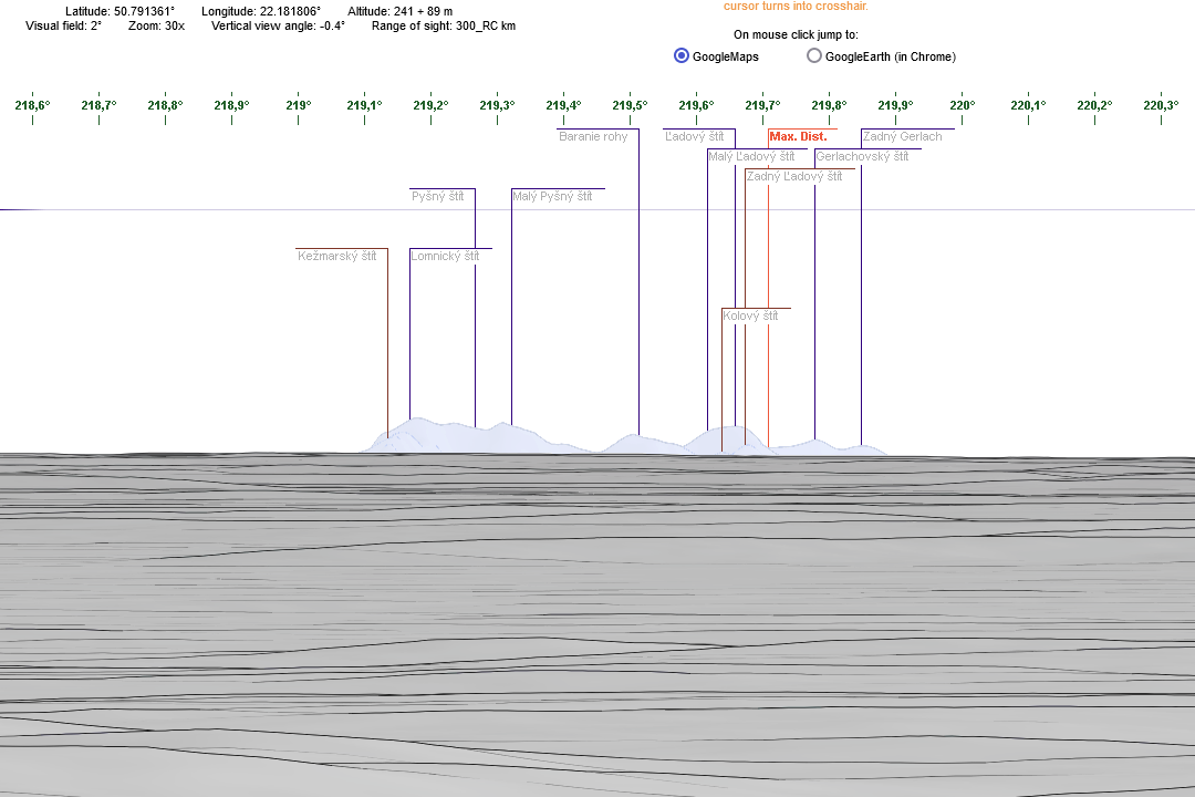
The view of the Tatra Mountains obtained by both methods looks quite similar, but several differences can be noted. These are due to the above-described features of the method with the observer’s elevation – only the relationship between Lomnica as well as peaks located at a similar distance and areas 52 km away is faithfully depicted. Therefore: farther peaks protrude slightly less, areas located farther than 52 km, but closer than the Tatra Mountains – too high, and areas located closer are mapped lower compared to the effect of refraction.
Let’s see how the refraction is simulated by increasing the height of the object at heywhatsthat.com. The maps there are generated for a standard refractive index of about 0.14, so differences from this value have been assumed for the calculations. The map on the left is created for an actual summit height of 2634 m above sea level, while the map on the right is for 2882 m above sea level – such an altitude, i.e. increased by 248 m, should reproduce a refraction of 0.22 compared to 0.14 for the observations from Potok Wielki (the distances to both points required in the calculations are the same as above).
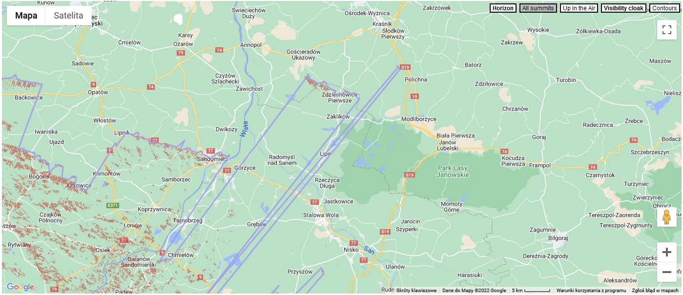
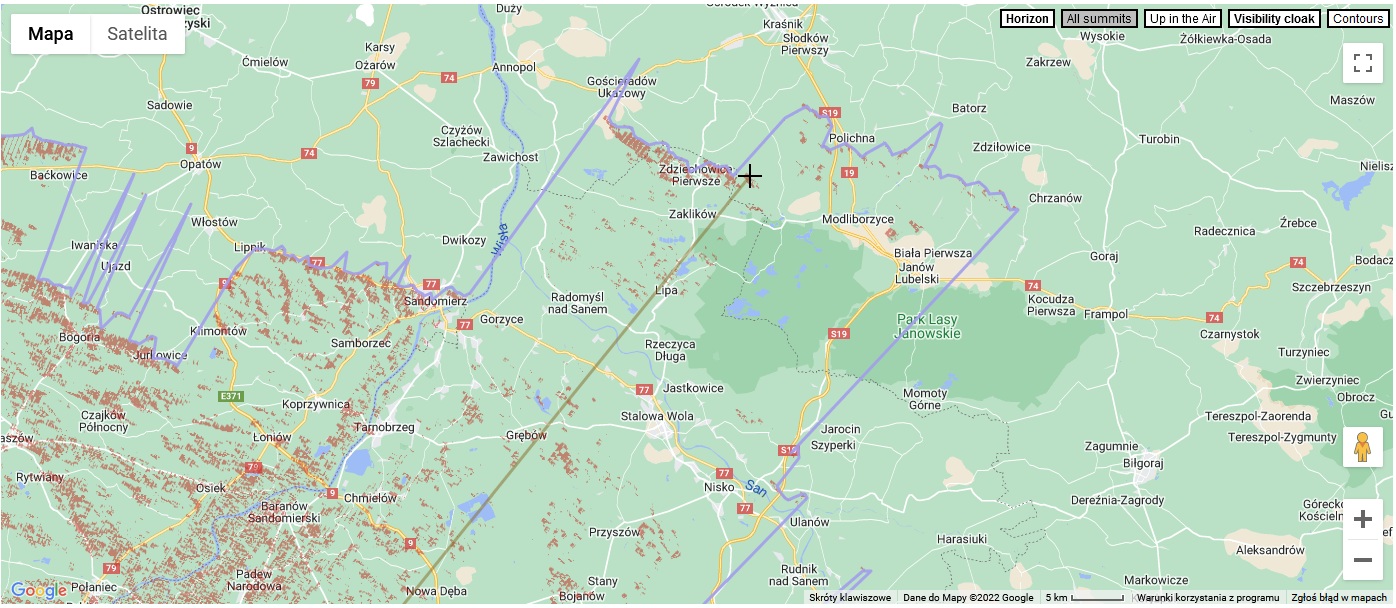
Increased altitude illustrates to some extent the range of visibility with increased refraction, but here there are also limitations related to distance. For more distant areas the refraction would be underestimated and for closer areas overestimated, the distance to the farthest visible area in front of the Tatra Mountains is also important. The method is therefore mainly applicable locally, to analyse visibility over a small area.
The profile below shows a comparison of the Lomnica observation line from Potok Wielki. The brown line is for a refraction coefficient of 0.22 and a peak height of 2634 m a.s.l., while the red line is for a coefficient of 0.14 and a peak height of 2882 m a.s.l. The lines intersect at a point 52 km from Potok, as the peak elevation was calculated in relation to this point.
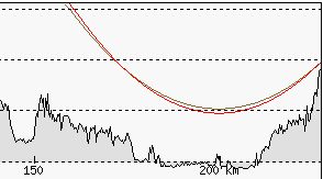
For a greater distance, the same refraction corresponds to a greater elevation of the object. This is the example of Lomnica as seen from the Romanian peak of Curcubăta Mare, 358 km away. The reference point was taken at a distance of 158 km – this is the farthest visible terrain obscuring Lomnica at standard refraction. Calculations show that simulating refraction with a coefficient of 0.22 requires an increase in the elevation of Lomnica by 450 m.
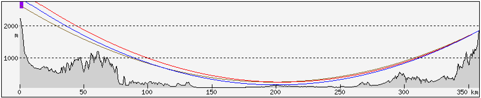
It can be seen that using the same elevation of Lomnica as for Potok Wielki does not correspond to the refraction relative to the selected reference point, located 158 km from the Romanian peak and 200 km from Lomnica – the blue line clearly deviates from the brown line at this point. The red line set to the summit of Lomnica raised by 450 m intersects the brown line at the selected point, so correctly reflects the influence of refraction relative to that point.